Training and Vizualizing Self Organizing Map(SOM) with Numerical Data
Published:
Recently i have started working in a cognitive science project. In our project, we wanted to use Self organising Map(SOM) for some cluster analysis purpose. While doing some research and implementation with SOM, i felt i could share my experience and learning with everyone and i will discuss step by step. I have implemented SOM with numerical dataset, the dataset is not so big either small. I will present and discuss the result a bit. Note: Data is not public , so not possible to share.
Let’s Talk about SOM a bit….
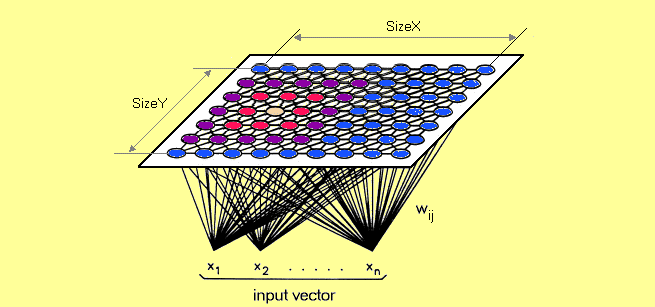
A self-organizing map (SOM) or self-organizing feature map (SOF) is a type of artificial neural network (ANN) that is trained using unsupervised learning to produce a low-dimensional (typically two-dimensional), discretized representation of the input space of the training samples, called a map, and is therefore a method to do dimensionality reduction. Self-organizing maps differ from other artificial neural networks as they apply competitive learning as opposed to error-correction learning (such as backpropagation with gradient descent), and in the sense that they use a neighborhood function to preserve the topological properties of the input space. This makes SOMs useful for visualization by creating low-dimensional views of high-dimensional data, akin to multidimensional scaling.

The artificial neural network introduced by the Finnish professor Teuvo Kohonen in the 1980s is sometimes called a Kohonen map or network.
SOM Algorithm:
Each data from data set recognizes themselves by competeting for representation. SOM mapping steps starts from initializing the weight vectors. From there a sample vector is selected randomly and the map of weight vectors is searched to find which weight best represents that sample. Each weight vector has neighboring weights that are close to it. The weight that is chosen is rewarded by being able to become more like that randomly selected sample vector. The neighbors of that weight are also rewarded by being able to become more like the chosen sample vector. From this step the number of neighbors and how much each weight can learn decreases over time. This whole process is repeated a large number of times, usually more than 1000 times.
In sum, learning occurs in several steps and over many iterations. :
1. Each node's weights are initialized.
2. A vector is chosen at random from the set of training data.
3. Every node is examined to calculate which one's weights are most like the input vector. The winning node is commonly known as the Best Matching Unit (BMU).
4. Then the neighbourhood of the BMU is calculated. The amount of neighbors decreases over time.
5. The winning weight is rewarded with becoming more like the sample vector. The nighbors also become more like the sample vector. The closer a node is to the BMU, the more its weights get altered and the farther away the neighbor is from the BMU, the less it learns.
6. Repeat step 2 for N iterations.
Best Matching Unit is a technique which calculates the distance from each weight to the sample vector, by running through all weight vectors. The weight with the shortest distance is the winner. There are numerous ways to determine the distance, however, the most commonly used method is the Euclidean Distance, and that’s what is used in the following implementation.
Implementation:
For my implementation, I have used a dataset which is consists of different metarials and the amoun of similarity among them. I am goign to find the similarities among those materials with SOM. The dataset has 21 materials with similaratites attributes, SOM will take the input and classify these materials into different class. I have tried 55 and 1010 grid. The grid is just nothing but a 2 dimensional vector.I have used Jupyter notebook for easy coding. Let’s code..
First take the input.
material_data=pd.read_csv("/home/hasan/../simdatawdT.csv").values
material_data=raw_data[:,1:]
print(material_data.shape)
Now set the network dimension and the number of iteration you want to train, i ahve set 10000 at first and the learning rate is 0.01.
network_dimensions = np.array([10, 10])
n_iterations = 10000
init_learning_rate = 0.01

normalise_data = True

# if True, assume all data on common scale
# if False, normalise to [0 1] range along each column
normalise_by_column = False
Now we initialize the neighbourhood radius and radius decay parameter.. how should the network reduce the radius.
# establish variables based on data
m = material_data.shape[0]
n = material_data.shape[1]
print(m)
# initial neighbourhood radius
init_radius = max(network_dimensions[0], network_dimensions[1]) / 2
# radius decay parameter
time_constant = n_iterations / np.log(init_radius)

data = material_data
Then we normalize the dataset if that is not normalize.
# check if data needs to be normalised
if normalise_data:
    if normalise_by_column:
        # normalise along each column
        col_maxes = raw_data.max(axis=0)
        data = raw_data / col_maxes[np.newaxis, :]
    else:
        # normalise entire dataset
        data = raw_data / data.max()
print(data)
The out put should be 2121 vector as my dataset is 2121 dimensional.
Sameple output:
[[1.0 0.17142857142857143 0.17142857142857143 0.17142857142857143
  0.2571428571428572 0.14285714285714285 0.2571428571428572
  0.14285714285714285 0.14285714285714285 0.19999999999999998
  0.2571428571428572 0.19999999999999998 0.17142857142857143
  0.34285714285714286 0.14285714285714285 0.42857142857142855
  0.14285714285714285 0.2857142857142857 0.31428571428571433
  0.14285714285714285 0.19999999999999998]
Now we will initialize some random weights for each row of the dataset and it should be m dimensional vector. The weights should be in between 0 and 1.
# setup random weights between 0 and 1
# weight matrix needs to be one m-dimensional vector for each neuron in the SOM
net = np.random.random((network_dimensions[0], network_dimensions[1], m))
print(net)
Sample output of the weights:
[[[0.94740172 0.81978749 0.66612662 ... 0.24751565 0.47871662 0.88681824]
  [0.30634451 0.80488439 0.95827778 ... 0.9796257  0.53824416 0.97624139]
  [0.74885045 0.47203416 0.99207747 ... 0.87340158 0.58623716 0.06587843]
  ...
  [0.33226436 0.88918553 0.95350665 ... 0.71388145 0.36370406 0.51415439]
  [0.28170385 0.28408134 0.68262441 ... 0.65870408 0.79460734 0.24192276]
  [0.89935803 0.74593964 0.93132826 ... 0.8555367  0.27766452 0.15437604]]
now, we will find the Best matching Unit(BMU) with the help of random weights we have initialized before, we just need to traverse through every row and calcualte the Euclidian distance between the weights of every node or neuron and every row of the dataset. Finally we will take the BMU index..
def find_bmu(t, net, m):
    """
        Find the best matching unit for a given vector, t, in the SOM
        Returns: a (bmu, bmu_idx) tuple where bmu is the high-dimensional BMU
                 and bmu_idx is the index of this vector in the SOM
    """
    bmu_idx = np.array([0, 0])
    # set the initial minimum distance to a huge number
    min_dist = np.iinfo(np.int).max
    # calculate the high-dimensional distance between each neuron and the input
    for x in range(net.shape[0]):
        for y in range(net.shape[1]):
            w = net[x, y, :].reshape(m, 1)
            # don't bother with actual Euclidean distance, to avoid expensive sqrt operation
            sq_dist = np.sum((w - t) ** 2)
            if sq_dist < min_dist:
                min_dist = sq_dist
                bmu_idx = np.array([x, y])
    # get vector corresponding to bmu_idx
    bmu = net[bmu_idx[0], bmu_idx[1], :].reshape(m, 1)
    # return the (bmu, bmu_idx) tuple
    return (bmu, bmu_idx)
Method for decaying radius, learning rate and calculating influence :
def decay_radius(initial_radius, i, time_constant):
    return initial_radius * np.exp(-i / time_constant)
def decay_learning_rate(initial_learning_rate, i, n_iterations):
    return initial_learning_rate * np.exp(-i / n_iterations)
def calculate_influence(distance, radius):
    return np.exp(-distance / (2* (radius**2)))
Now we will take randomly each data and calculate the Euclidian distance to find the BMU , then we will update the weight of this neuron…We will use BMU method for this…
for i in range(n_iterations):
    #print('Iteration %d' % i)

    # select a training example at random
    t = data[:, np.random.randint(0, n)].reshape(np.array([m, 1]))
    #print("first t value:", t);

    # find its Best Matching Unit
    bmu, bmu_idx = find_bmu(t, net, m)
    #print("bmu_index: ",bmu_idx)

    # decay the SOM parameters
    r = decay_radius(init_radius, i, time_constant)
    l = decay_learning_rate(init_learning_rate, i, n_iterations)

    # now we know the BMU, update its weight vector to move closer to input
    # and move its neighbours in 2-D space closer
    # by a factor proportional to their 2-D distance from the BMU
    for x in range(net.shape[0]):
        for y in range(net.shape[1]):
            w = net[x, y, :].reshape(m, 1)

            #print("net",net)
            #print("wwww:",w)
            # get the 2-D distance (again, not the actual Euclidean distance)
            w_dist = np.sum((np.array([x, y]) - bmu_idx) ** 2)
            # if the distance is within the current neighbourhood radius
            if w_dist <= r**2:
                # calculate the degree of influence (based on the 2-D distance)
                influence = calculate_influence(w_dist, r)
                # now update the neuron's weight using the formula:
                # new w = old w + (learning rate * influence * delta)
                # where delta = input vector (t) - old w
                new_w = w + (l * influence * (t - w))
                # commit the new weight
                net[x, y, :] = new_w.reshape(1, 21)
These are my materials name from my dataset:
material_nams=\
["Adhesive","Brick","Cardboard","Ceramic","Cloth","Concrete","Cotton","Diamond","Glass","Leather","Marble","Metal","Paper","Plastic","Porcelain","Rubber","Stone","Styrofoam","Wax","Wood","Wool"]
To make the final classification we will take the final weight of the nodes and divide each data from the dataset to know about which class it belongs to…
def find_classification(t, net, m):
    bmu_idx = np.array([0, 0])
    # set the initial minimum distance to a huge number
    min_dist = np.iinfo(np.int).max
    # calculate the high-dimensional distance between each neuron and the input
    for x in range(net.shape[0]):
        for y in range(net.shape[1]):
            w = net[x, y, :].reshape(m, 1)
            # don't bother with actual Euclidean distance, to avoid expensive sqrt operation
            sq_dist = np.sum((w - t) ** 2)
            if sq_dist < min_dist:
                min_dist = sq_dist
                bmu_idx = np.array([x, y])
    # get vector corresponding to bmu_idx
    bmu = net[bmu_idx[0], bmu_idx[1], :].reshape(m, 1)
    # return the (bmu, bmu_idx) tuple
    return (bmu, bmu_idx)
After that we will get the index of the each BMU of each material and we can find the position of each material in the graph… sample putput is like this..
bmu_index:  [1 2]
bmu_index:  [2 3]
bmu_index:  [2 2]
bmu_index:  [1 2]
bmu_index:  [1 1]
bmu_index:  [2 3]
bmu_index:  [1 1]
bmu_index:  [2 3]
bmu_index:  [2 3]
bmu_index:  [1 1]
bmu_index:  [1 2]
bmu_index:  [2 3]
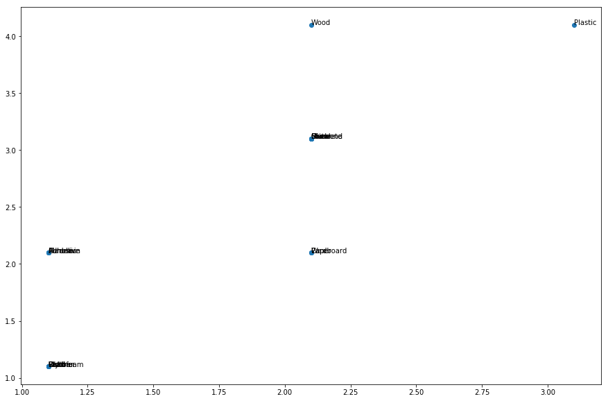
Now we want to visualize our result what we got so far… For 5 by 5 size SOM :
print("Graph for 5*5 size SOM")
    #print(m[1])

    #print("m10:",list1[1])
    #plt.text(list1,list2, material_nams[i], ha='center', va='center',
     #    bbox=dict(facecolor='white', alpha=1, lw=0))

f = plt.figure(figsize=(15,10))
ax = f.subplots()
ax.scatter(list3, list4)

for i, txt in enumerate(material_nams):

    ax.annotate(txt, (list3[i], list4[i]))
    list3[i]+=0.3
    list4[i]+=0.3
If we see the result in 2D: 
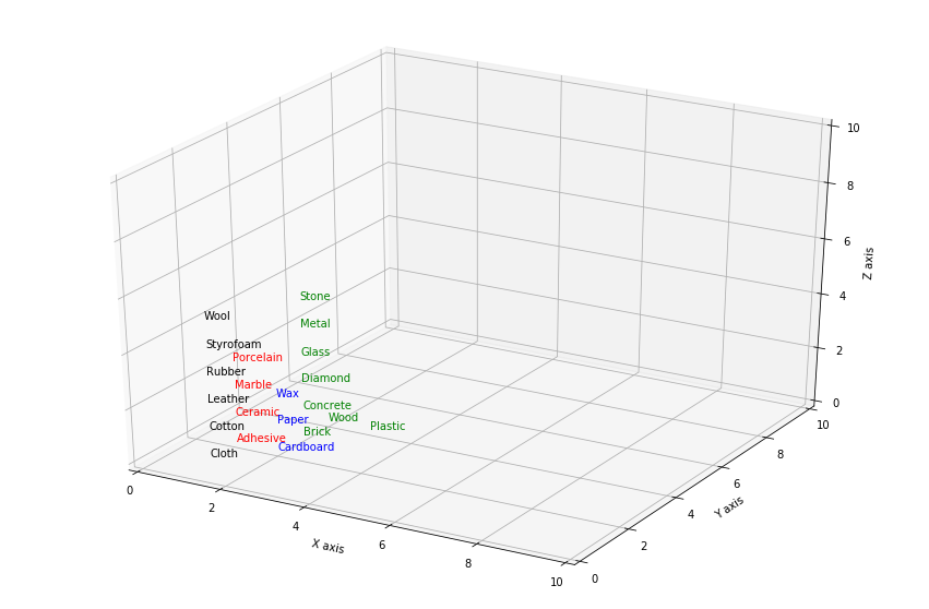
As we can see that some node has more than one materials as the attributes are similar of these materials , As we can not clearly see the materials name, we can show it in 3D:

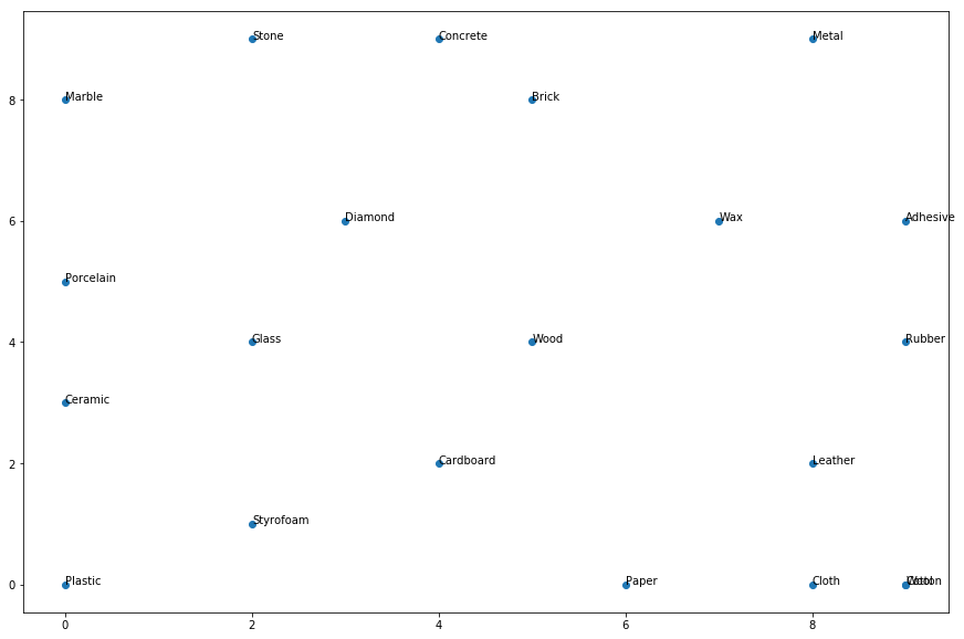
For 10*10 graph , we can visualize the graph by following way:
print("Graph for 10*10 size SOM")
f = plt.figure(figsize=(15,10))
ax = f.subplots()
ax.scatter(list1, list2)

for i, txt in enumerate(material_nams):

    ax.annotate(txt, (list1[i], list2[i]))
From the foloowing 2D graph we can how all the materials has been clustered in dfferent nodes, We can see similar material are set beside each other. More similar mean more close and less similar means more distance.

Now, we can easily understand from this output, how SOM clustered object and how powerful this neural network is. This can be used for plenty of scenario where cluster analysis is important.
References:
- https://en.wikipedia.org/wiki/Self-organizing_map
- https://towardsdatascience.com/self-organizing-maps-ff5853a118d4
- http://www.pitt.edu/~is2470pb/Spring05/FinalProjects/Group1a/tutorial/som.html
